1/7: Introduction

This article is part of a series on performance guidelines.

After spending a long time answering the same questions, over and over again, about performance techniques on CPUs and, lately, on GPUs, I decided to write this text using sorting algorithms as an example, since their proper implementation will force us to review all the fundamental directives needed for writing performance-optimized code. Even though sorting algorithms are at the core of this discussion, it turns out that all of the techniques described will apply to nearly every class of algorithm.

Throughout this text, N is the problem’s input size.

Fundamental concepts

To make any significant headway into this text, the reader should already be familiar with the fundamental concepts behind GPU programming, preferably having already written parallel code. The CUDA Toolkit’s “C Programming Guide” is an excellent starting point. Knowledge of the basics on computational complexity is also required.

CUDAfy.NET

All sample source code is written in C#, using CUDAfy for all GPU-bound code.

“CUDAfy .NET allows easy development of high performance GPGPU applications completely from the Microsoft .NET framework”

Before I used CUDAfy, I had to wrap my C code within a static library and link it against my .NET application, which led to a significant effort in code maintenance and the annoyance of dealing with two languages simultaneously. With CUDAfy I can write CPU and GPU code directly in C#, inside the same assembly and without ever leaving my visual studio project. Except for very contrived scenarios, everything I used to be able to do in C can now be done in C# without loss of functionality. In spite of its name, CUDAfy can not only interface with the GPU through CUDA, but also via OpenCL, allowing the developer to target most architectures at will from the same C# code with (barely) no modifications.

Language and Compiler choice

The first step most programmers usually take while tuning performance is to use a lower level language (ex. C++ vs C#) on their inner loops, usually gaining approximately a 10% to 20% speed improvement with the correct compiler settings. But there’s so much gain to be had elsewhere that it’s the last thing I usually do. Rewriting your inner loop in a different language, and setting up a parallel project to link against is time consuming, error prone and will lead to a greater effort in code maintenance. Do yourself a favour and leave it for last.

GPU nomenclature

Throughout this text I’ll use NVIDIA/CUDA terms such as warps (vs Wavefronts for AMD), shared memory (vs Local Memory for OpenCL), etc. But in nearly every case, your favourite GPU architecture will have concepts that match CUDA’s. Everything written herein applies only for NVIDIA architectures with compute >= 2.0.

Diminishing returns

It may seem odd giving such an advice on a document about improving performance, but I have seen this behaviour so often that I felt the need to make my point early on:

Don’t overdo it. Focus your valuable engineer time on that which may give the greater returns on your investment. Work only on your inner loops, where the performance gains are greatest. Why spend weeks optimizing the rest of a piece of software for a measly 5% speed improvement when you can really tune the inner loop of your algorithms and gain a whooping 50%? Prioritize, and know when to quit.

2/7: The CPU memory cache

This article is part of a series on performance guidelines.

Nearly every developer is at least vaguely aware of the existence of a caching system on most modern computers, but not many actually program their inner loops and algorithms with it in mind. And yet, once algorithmic complexity considerations are resolved, memory cache should become the main focus while trying to increase a program’s performance.

While a typical CPU instruction can take, on average, one clock cycle (sometimes a lot less), uncached memory access can easily take between 50 and 100 clock cycles (this ratio has been increasing over the years, since CPU clock frequency, driven by market forces, has raised faster than memory speed and bus bandwidth). These days, accessing memory can easily be 100 times slower than executing one single typical assembly instruction. There’s a lot of room for improvement here by working with the memory cache, and not against it.

Architecture

In this diagram of a pseudo-CPU memory access model, the arrows represent dataflow paths, the thicker the arrow, the wider the flow capacity. Usually L1 memory resides on the same core; L2 cache is usually on-chip and may either reside within each core, or is shared between them; L3 cache, if at all present, may either be on or off-chip. L1 cache is the fastest and usually the tiniest, while L3 has the greatest capacity and is the slowest.

A simple guideline

While the greatest performance gains may only be achieved by knowing the exact cache characteristics of the CPU we’re programming against (look-aside vs look-through, write policies, cache line and cache page sizes, cache organization – fully associative vs direct map, etc), in the vast majority of cases we can get excellent results by following a simple guideline:

Make sure your algorithm accesses only the same small regions of data for as long as possible before moving elsewhere.

Programming techniques – loop blocking

A simple programming technique to achieve this goal is loop blocking: Divide your data-scanning loops into coupled sub-loops and reorder them within the hierarchy of nested loops. Here’s a typical example, for a matrix square product (X.Y=Z):

1 – Trivial implementation

for (int I = 0; I < M; I++)

   for (int K = 0; K < M; K++)

      for (int J = 0; J < M; J++)

         Z[J, I] = Z[J, I] + X[K, I] * Y[J, K];

2 – Loop split, for block size B <= M

for (int I = 0; I < M; I++)

   // K loop, part 1

   for (int K2 = 0; K2 < M; K2 += B)

      // K loop, part 2

      for (int K1 = K2; K1 < Math.Min(K2 + B, M); K1++)

         // J loop, part 1

         for (int J2 = 0; J2 < M; J2 += B)

            // J loop, part 2

            for (int J1 = J2; J1 < Math.Min(J2 + B, M); J1++)

               Z[J1, I] = Z[J1, I] + X[K1, I] * Y[J1, K1];

3 – Reordered loops, becoming cache-optimized

// K loop, part 1, reordered

for (int K2 = 0; K2 < M; K2 += B)

   // J loop, part 1, reordered

   for (int J2 = 0; J2 < M; J2 += B)

      for (int I = 0; I < M; I++) // reordered I loop

         // K loop, part 2, reordered

         for (int K1 = K2; K1 < Math.Min(K2 + B, M); K1++)

            // J loop, part 2, reordered

            for (int J1 = J2; J1 < Math.Min(J2 + B, M); J1++)

               Z[J1, I] = Z[J1, I] + X[K1, I] * Y[J1, K1];

Given the varying nature of the underlying hardware’s architecture, the best choice for the block size “B” must be empirically determined over a range of reasonable values.

Other similar techniques exist, variations on the method above.

Programming techniques – memory buffer layout

The way data is laid out onto memory may affect cache performance. As an example, consider the following two schemes for storing key/value 32-bit word pairs:

1 – Two uint[] arrays, one holding the sequence of keys, the other the corresponding sequence of values. Useful when using algorithms that iterate over either the key array or the value array, but not both at once. For example, computing the maximum of the value array. This way, no unnecessary memory elements are loaded.

uint[] keys, values;

2 – An array of key/value pair structs. Used when both key and value are needed within each inner loop iteration - for example, when sorting the array. Whenever a key is loaded from memory it’s likely that, due to proximity, the corresponding value has also been loaded into cache, resulting in a cache hit once it’s requested.

public struct kvp

{

public uint key;

public uint value;

}

kvp[] kvps;

3/7: Algorithmic performance

This article is part of a series on performance guidelines.

We shall walk the steps needed to choose the right algorithm for a particular task. These steps are ordered from the most to the least important. Even though written with sorting algorithms in mind, most of these topics are relevant regardless of the algorithm’s nature.

Temporal complexity

Above all other considerations, the search for the right algorithm to a particular problem should focus on worst-case temporal computational complexity. Indeed, in real-world large scale applications, the mere possibility that a contrived input vector may bring the whole system down to a crawl is simply not acceptable, no matter how unlikely. Every mainstream algorithm has been studied throughout and its worst-case complexity made known, so there is really no excuse to use an uninformed choice.

Locality

Of course, there’s a long distance from theory to practice, and one often finds that algorithms exhibiting very good asymptotic complexity turn out to have a very bad performance once implemented in a specific real-world scenario. We’ll see a good practical example of this effect in our last chapter.

For example, when working with a relatively small problem size N, the choice between Quicksort and heapsort isn’t exactly trivial. At first sight, heapsort should win hands-down, since it has a much better O(n*Log(n)) worst-case temporal complexity when compared to quicksort’s O(n^2). But another aspect comes into play – space and temporal locality. Quicksort tends to work for long periods on relatively small patches of memory, which means that a cached memory bank, once loaded, will be thoroughly exploited by the algorithm, before it moves its focus elsewhere in the input array. In contrast, heapsort accesses memory all over the place, with no apparent rhyme or reason. It’s a nightmare from a caching standpoint. This has such a great impact on performance that quicksort will end up being faster. Of course, once one enters the realm of large data sets, the n-squared algorithmic complexity quickly raises its ugly head and quicksort soon loses its advantage.

The same can be said of radix sort – its linear temporal complexity only becomes relevant for significantly large data sets, due to a fairly large constant multiplicative factor on top of the linear complexity, coupled with it being very cache unfriendly.

Space complexity

Once we’ve decided on a subset of algorithms, the next factor that will help us make the final decision is space complexity. When space is at a premium, we may not be able to afford the extra temporary storage that many sorting algorithms use. For example, a cache-optimized mergesort is by far the best jack-of-all-trades sorting algorithm, exhibiting superb performance together with sorting stability (a sorting algorithm is said to be stable when the original relative position of identical keys is preserved on the sorted list). Alas, mergesort needs temporary storage of the same size as the original list, which isn’t much of a problem in these days and age when CPU RAM is cheap. But in specialized hardware, such as a GPU, memory is still at a premium, which may condition algorithm choice.

Best case performance

In many cases, the specifics of our problem at hand may give us additional guidelines in our algorithm choice. For example, if we know that in most cases our lists are nearly sorted, then we could have significant improvements if we chose an algorithm with a linear-time best case for already sorted lists, such as Insertion sort (if our lists are really small) or smoothsort (if locality isn’t a big problem).

Stability

Stability is often a desirable intrinsic property of a sorting algorithm. In practice, a non-stable algorithm can be made stable by adding a secondary indexer to be used when resolving disputed comparisons with identical keys. While requiring twice as much memory, this addition doesn’t increase the asymptotic temporal complexity, so in many cases it’s an acceptable trade-off.

4/7: The GPU – a performance-centric overview

This article is part of a series on performance guidelines.

Ask most programmers without previous GPU programming experience how they’d go about writing a parallel sorting algorithm, and most will tentatively forward the same approach: subdivide your unsorted list into small chunks, and have each thread process them individually using a standard linear sorting algorithm (usually quicksort – people love quicksort), somehow magically merging the small sorted lists into our output list. This won’t work, and to understand why we need to focus on how memory access and caching is handled in a typical GPU.

Architecture

Like a CPU, the GPU memory model has Level 1 and 2 caches (hence a need for locality) but a much heftier penalty for a cache miss. For example, for a Fermi card, expect a few clock cycles for shared memory / L1 access and potentially hundreds of cycles for off-chip global memory access.

Usually the L1 cache is held within each SM (Streaming Multiprocessor), while the L2 banks are shared. The memory interface is fairly wide (for a Fermi card, for instance, its 384-bit wide, allowing for 12 contiguous 32-bit words to be fetch from memory at once per ½ clock cycle).

Finally, the PCI Express bus bridges access between the GPU and the host memory, resulting in another layer of indirection and possible bottleneck. Moving memory between host and device can be approximately one order of magnitude slower than on-device memory access.

Shared memory

Besides L1 storage, the SM’s on-chip memory is also used as shared memory, visible by all threads within a block. Shared memory’s usage pattern is as a staging area for global memory load and storage; in other words, instead of relying on the L1 cache’s algorithms to decide what to cache and what to skip, the programmer uses shared memory to get precise control over what gets stored in the L1 memory banks. Of course, the more memory we explicitly allocate as shared memory, the less we have for L1, and vice-versa.

Bank conflicts

Shared memory is distributed across a number of equally-sized banks, usually as many as the warp size; contiguous elements in a shared memory buffer will be stored in contiguous banks. Since each bank can process only one memory access per clock cycle (multicasting as needed, serving several threads within a warp requesting the same index), if more than one thread in the warp accesses different indexes within the same block then a bank conflict happens, where each thread access is serialized, resulting in performance degradation. Simply put:

In a given clock cycle and for any threads A and B within the same warp: if thread A accesses shared memory index X and thread B accesses index X+U*32, for any X and any U!=0, then a bank conflict will happen.

Coalesced global memory access

We’ve already established just how costly global memory access can be. But at times it just can’t be helped, for instance, when loading global memory to a temporary storage buffer in shared memory used for further computations.

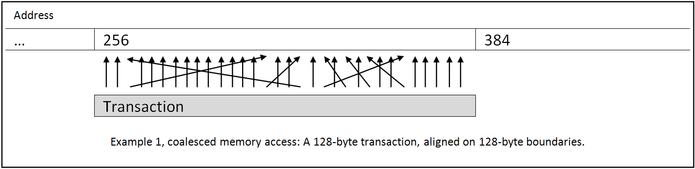
Each global memory access is packed into a contiguous 128 byte transaction (on recent architectures). Such transactions will read exactly 128 bytes from a 128 byte-aligned buffer in global memory. The transaction itself is also aligned on 128 byte-boundaries.

Ideally each thread in a warp participates in the request, specifying which part of a contiguous 128 bytes block in global memory it will be accessing. In the end, all the threads in the warp will be serviced by a single transaction (4 bytes * 32 threads = 128 bytes).

If each thread reads more than a 32-bit word, or if the addresses requested extend beyond a 128 byte-aligned buffer, more transactions need to be issued (with separate transactions for each separate 128-byte line that is touched). The particular index within the 128-byte segment accessed by each thread in a warp is no longer relevant for recent GPU architectures (but for backward compatibility, the access should be sequential).

Because of these restrictions, it is often good practice padding the end of data structures in order to preserve the 128-byte alignment. For example, bidimensional arrays stored in a contiguous buffer may need extra padding at the end of each row, ensuring that the next row begins at a 128-byte boundary.

Memory access guidelines

Let’s now revisit our naïf parallel sorting algorithm: picture thousands of threads, each pseudo-randomly accessing memory, oblivious of what the other threads are doing. Given a large enough problem size, practically all of those memory accesses will naturally result in cache misses, and each of these individual accesses would waste 120 bytes on each corresponding transaction. We can imagine the memory interface as a 384-bit wide keyhole, beyond which all threads are piling up, idly waiting for their turn to wastefully access memory. Our naïf sorting algorithm is in fact a linear algorithm.

 This applies not only to sorting algorithms, but to a vast class of problems. Due to its serial nature, it turns out that

Memory access is possibly the greatest bottleneck of parallel computing.

To work around the memory access limitation, we have to design our algorithms so that

1.      Every thread within a block should work with the same small memory buffer, for as long as possible, before discarding it. This buffer should reside in shared memory, which uses the same fast memory as the L1 cache.

2.      Global memory accesses within a warp should be coalesced.

3.      Shared memory bank conflicts should be avoided.

4.      All the cache programming techniques discussed previously for CPUs (like blocking) also apply for GPUs, and are even more relevant given GPU memory access’s central stage.

5.      Avoid frequent host memory access. Move the data once onto the device, and keep it there. If you must move it, do it simultaneously with another operation, such as running a kernel on the GPU.

Warp divergence

Once the memory access problem has been satisfactorily solved, another aspect to optimize is the divergence within a warp. All threads within a warp usually march in lockstep, each processing exactly the same instruction in the same clock cycle. When they don’t we have a divergence, i.e., a situation where the warp’s threads are forced to run different execution paths, usually as a consequence of an “if” or a “case”. The way the SM handles such divergent paths is to serialize their execution, keeping every unused thread within the warp idle and thereby wasting resources.

Imagine the following instruction being processed within a warp:

if (threadIx < 16)

    myVar = 0;

else

    myVar = 16;

Within a 32-thread warp, the flow of events is:

1 – All threads process the conditional instruction;

2 – The threads 0 to 15 will assign their register, while the remaining threads will stay idle;

3 - The threads 0 to 15 will stay idle, while the remaining threads will assign the register.

But we can eliminate the divergence altogether if instead we write

myVar = (threadIx & 0x10);

At the very least, one should try not to split warps by conditional instructions. The following would be acceptable:

if (threadIx < 32)

    myOtherVar *= 2;

else

    myOtherVar = 0;

Because warp #1 processes the product by 2, while all remaining warps assign 0 to the register, there’s no need for warp divergences and therefore no threads are idle within the block.

Register spillage

Each thread has a limited number of registers available to execute a program’s logic (usually, up to 32 per thread, on a modern architecture), which is a potential bottleneck. The compiler will try its best to reuse the registers as much as possible, but for some more complex algorithms it simply won’t do. Once more than 32 registers are needed, L1 memory storage will be hijacked to emulate additional registers, but with an obvious performance impact. The worst happens when even the L1 isn’t enough to accommodate our program’s requirements and the GPU is forced to use global memory to hold register values. At this point the performance will degrade enormously, which should be avoided at all costs, usually by reorganizing an algorithm’s code through clever programming.

5/7: Sorting algorithms on a GPU

This article is part of a series on performance guidelines.

We’ve seen how important it is that threads in a warp work together while accessing device memory. To that effect, one has to abandon the notion of threads acting on their own, so familiar with CPU programming, and use instead the block or the warp as the primary unit of work, where its underlying threads are mere cogs of a larger machine. I find that it helps when I mentally picture the warp as a woven fabric whose threads are either the loom’s needles or the fabric’s mesh. As an example, consider the following graphical representation of a well-known parallel sorting algorithm – Batcher’s Bitonic Sort – applied to an array of 32 elements.

Each horizontal line represents an index of the length 32 buffer to be sorted; each arrow depicts a thread performing a “compare-and-swap” operation on two memory indexes – two values are compared and, if the inequality holds, swapped.

This class of algorithms (called Sorting Networks) has the characteristic that at any point in time, each thread’s actions are independent from any previous action of any thread. This is an important feature since transferring information between warps within a parallel setup can often be expensive in terms of synchronization. Also, it makes it possible to represent the algorithm through a diagram such as the one pictured above.

The diagram is split into columns (A to O) so that all threads within each column may act in unison without risking a race condition.

Bitonic Sort

For Batcher’s Bitonic Sort, it turns out that each column always uses the same number of threads – precisely half the number of indexes in the buffer – and that powers of two are ubiquitous, implying a significant speed boost for many arithmetic operations.

There is also an obvious compartmentalization of buffer access that we can exploit to take advantage of the memory access pattern for GPUs:

Let’s, for the sake of the argument, assume we are using the above diagram to sort a list of 32-bit words using a GPU with a warp size of 8 and a shared memory maximum size of 16 32-bit words per warp. Therefore we’d need to use two warps working concurrently to sort this list, which we’ll call Warp1 and Warp2. We’ll assign the sorting buffer’s indexes 0 through 15 to Warp1 and indexes 16 through 31 to Warp2. Under this setup, if each warp loads the values of their assigned indexes into their respective shared memory buffer, they will be able to work exclusively with shared memory right to the point when the threads reach column K. At this juncture, each warp has no alternative but to store the result of their computations back into global memory, making it visible to the remaining warps. Even though we can’t use shared memory while processing column K, we can at least have coalesced global memory access, since the indexes to be accessed are all sequential and aligned in power-of-two boundaries. Once column K is processed, we can revert to our original method of using shared memory as temporary storage until our list is fully sorted. We have, therefore, used two distinct algorithms for different stages of the sorting – one using shared memory, the other enforcing coalesced global memory access. Unfortunately, we can’t seem to avoid shared memory bank conflicts, as can be easily seen by examining, for instance, column H, where thread #0 in Warp1 accesses Bank 0 to read index 0 and thread #4 also accesses Bank 0 to read index 8 (because there are 8 banks, as many as the warp size, and 0 == 8 % 8).

We conclude that the Bitonic Sort algorithm exhibits good locality and good use of warp resources. But it also has problems with bank access violations and isn’t always able to use shared memory as a means to avoid reading from global memory, particularly as the array size becomes larger.

Odd-Even Merge Sort

When it comes to algorithmic complexity, it turns out that the best general-purpose sorting network (i.e., which works for an arbitrary input array size) is Batcher’s Odd-Even Merge Sort (apart from some theoretical work with no practical implementation), with its
¼*n*Log(n)*(Log(n)-1)+n-1 instructions, comparing favourably against Bitonic’s
¼*n*Log(n)*(Log(n)+1) instructions. While both have a worst case complexity of O(n*Log(n)^2), their hidden constants can still play a significant part in our decision process.

That, unfortunately, is its only advantage against Bitonic Sort, since features such as full-warp utilization, spatial locality and shared memory pattern only apply at the very beginning of the sorting process, when the memory access per warp is still properly segmented.

Performance comparison

# Rows	Bitonic (ms)	Oddeven (ms)
16K	0.47	1.20
32K	0.53	1.39
64K	0.71	1.70
128K	0.75	2.01
256K	0.80	2.32
512K	1.07	6.47
1M	4.49	14.71
2M	12.15	33.64
4M	30.27	75.34
8M	72.95	169.90
16M	173.42	382.45
32M	405.50	848.96
64M	932.00	1875.55

Is the lower worst-case complexity still a good enough justification to choose it over Bitonic sort? To find out, I adapted NVIDIA’s CUDA Toolkit’s samples to CUDAfy and ran some tests on a GeForce 680 GTX. The charted times are in milliseconds, and the test run times were averaged over 100 repetitions, after an adequate warm-up period. Another chart plots the exact number of compare-and-swap operations for both sorting algorithms. Both charts are in Logarithmic (base 2) scale. The Size of List is measured in number of list elements, where each element is a 32-bit pair of key-value; for example, a list size of 512K will result in an underlying buffer of exactly 4 megabytes

As it turns out, our implementation of Bitonic sort wins for array lengths of up to 64 million, in spite of a larger constant factor on the algorithmic complexity, clearly showing how important is the memory access design patterns previously discussed.

It's also worth noticing the slope in the vicinity of the 256K list size, and one can't help wondering if it is in any way related with the GTX 680's L2 cache size of 512KB. A list of 256*1024 elements fits exactly in 2MB, for times the size of the L2 cache. Even though the whole list will no longer fit fully in the L2 cache, the cache's hit/miss ratio will still remain fairly high for buffers that won't far exceed the L2 cache's size. This effect will drop sharply once the buffer becomes too large for the L2.

Further considerations

Sorting Networks aren’t the only choice available when it comes to parallel implementations, but they certainly are the most enticing. Although viable alternatives exist, such as parallel radix sort (implemented in thrust library’s adaptive sort, for example), they are either too dependent on the data type being sorted, are fiendishly complex to implement or have poor locality (usually it’s all of the above).

The Log-squared limitation on Sorting Networks isn’t really very important given that it only becomes a factor with very large array sizes, usually beyond the memory available in typical desktop GPUs.

Given the prohibitively slow data transfer rate between host and device, usually one only sorts arrays on the GPU as part of a larger GPU-bound algorithm. Otherwise it would be simpler to just sort on the CPU and do away with the additional memory transfers. Unless, that is, we opt for the extra complexity of a hybrid CPU-GPU sorter, where 3 distinct operations are simultaneously carried out:

1 – The GPU sorts small to medium-sized arrays;

2 – The CPU merges the already sorted arrays from (1);

3 – Memory is transferred between host-device. This step may be further subdivided in two distinct lanes, one copying data to be sorted onto the device, while the other copies sorted data back to the host.

Each of these steps may happen simultaneously because they use different resources – the GPU, the CPU and the PICe bus. The hybrid approach also has the advantage of easily fixing the lack of a straightforward implementation of GPU sorting for non-powers of two, by delegating on the CPU the sorting of the non-power-of-two leftover arrays and their subsequent merge with the GPU-sorted power-of-two arrays:

1 – Split the list into a larger power-of-two list A and a smaller list B with the remainder.

2 – Sort A normally on the GPU.

3 – Either sort B on the CPU, or apply step (1) recursively until the remainder is small enough to be sorted on the CPU.

4 – Merge the sorted lists together on the CPU.

7/7: Apendix B – CUDAfy source for Bitonic sort

This article is part of a series on performance guidelines.

/* 
 * This software is based upon the book CUDA By Example by Sanders and Kandrot.
 * This software contains source code provided by NVIDIA Corporation.
*/

/* Original Copyright notice:
 * Copyright 1993-2012 NVIDIA Corporation.  All rights reserved.
 *
 * Please refer to the NVIDIA end user license agreement (EULA) associated
 * with this source code for terms and conditions that govern your use of
 * this software. Any use, reproduction, disclosure, or distribution of
 * this software and related documentation outside the terms of the EULA
 * is strictly prohibited.
 *
 */

public static class bitonic
{
  private static bool IsPow2(uint i)
  {
    return i > 0 && i == (i & ~(i - 1));
  }

  public static void DoBitonicSort(GPGPU gpu, KVP[] d_kvp, bool SortAsc)
  {
    uint dir = (SortAsc ? 1U : 0);
    int arrayLength = gpu.GetDeviceMemory(d_kvp).XSize;

    if (!IsPow2((uint)arrayLength))
      throw new ApplicationException("Invalid array length. Must be a power of 2.");
    if (!IsPow2(SHARED_SIZE_LIMIT))
      throw new ApplicationException("Invalid SHARED_SIZE_LIMIT length. Must be a power of 2.");
    if (arrayLength <= SHARED_SIZE_LIMIT)
      throw new ApplicationException("Invalid array length. Must greater than SHARED_SIZE_LIMIT");
    int CorrectKVPLengthUint = Marshal.SizeOf(typeof(KVP)) / Marshal.SizeOf(typeof(uint));
    if (CorrectKVPLengthUint != KVPLengthUint)
      throw new ApplicationException(string.Format(
        "KVPLengthUint ({0}) must equal the size of KVP in uint's ({1})", KVPLengthUint, CorrectKVPLengthUint));

    int blockCount = arrayLength / (int)SHARED_SIZE_LIMIT;
    int mergeGlobalBlockCount = 2 * blockCount;
    int mergeGlobalThreadCount = threadCount / 2;

    gpu.Launch(blockCount, threadCount, bitonicSortShared1, d_kvp);

    for (uint size = 2 * SHARED_SIZE_LIMIT; size <= arrayLength; size <<= 1)
      for (uint stride = size / 2; stride > 0; stride >>= 1)
        if (stride >= SHARED_SIZE_LIMIT)
        {
          gpu.Launch(mergeGlobalBlockCount, mergeGlobalThreadCount, bitonicMergeGlobal, d_kvp, size, stride, dir);
        }
        else
        {
          gpu.Launch(blockCount, threadCount, bitonicMergeShared, d_kvp, size, dir);
          break;
        }
  }

  public const uint SHARED_SIZE_LIMIT = 2U * threadCount;
  public const int threadCount = 512;
  public const uint KVPLengthUint = 2U;

  [Cudafy]
  public struct KVP
  {
    //public uint key;
    public uint key, value;

    [CudafyIgnore]
    public override string ToString()
    {
      //return String.Format("{0}", key);
      return String.Format("{0},{1}", key, value);
    }

    [CudafyIgnore]
    public override bool Equals(object obj)
    {
      return ((KVP)obj).key == key;
    }

    [CudafyIgnore]
    public override int GetHashCode()
    {
      return (int)key;
    }
  }

  [Cudafy(eCudafyType.Device)]
  public static void Comparator(
      ref KVP A,
      ref KVP B,
      uint dir)
  {
    KVP tmp;
    if (dir == 0 && (A.key < B.key) || dir != 0 && (A.key > B.key))
    {
      tmp = A;
      A = B;
      B = tmp;
    }
  }

  [Cudafy]
  private unsafe static void bitonicSortShared1(GThread thread, KVP[] d_kvp)
  {
    //Shared memory storage for current subarray
    KVP[] s_kvp = thread.AllocateShared<KVP>("s_kvp", (int)SHARED_SIZE_LIMIT);
    fixed (KVP* s_Ptr_kvp = s_kvp)
    fixed (KVP* d_Ptr_kvp = d_kvp)
    {
      int tid = thread.threadIdx.x;

      //Offset to the beginning of subarray and load data, in coalesced batches
      uint* d_Ptr_kvp_offset = (uint*)(d_Ptr_kvp) + ((uint)thread.blockIdx.x * SHARED_SIZE_LIMIT) * KVPLengthUint;
      for (int bbIx = 0, offset = 0; bbIx < KVPLengthUint * 2; bbIx++, offset += threadCount)
        ((uint*)(s_Ptr_kvp))[tid + offset] = d_Ptr_kvp_offset[tid + offset];

      for (uint size = 2; size < SHARED_SIZE_LIMIT; size <<= 1)
      {
        uint ddd = ((tid & (size / 2))) != 0 ? 1U : 0;

        for (uint stride = size / 2; stride > 0; stride >>= 1)
        {
          thread.SyncThreads();
          uint pos = 2 * (uint)tid - ((uint)tid & (stride - 1));
          Comparator(ref (s_kvp[pos + 0]), ref (s_kvp[pos + stride]), ddd);
        }
      }

      {
        uint ddd = (uint)thread.blockIdx.x & 1;
        for (uint stride = SHARED_SIZE_LIMIT / 2; stride > 0; stride >>= 1)
        {
          thread.SyncThreads();
          uint pos = 2 * (uint)tid - ((uint)tid & (stride - 1));
          Comparator(ref (s_kvp[pos + 0]), ref (s_kvp[pos + stride]), ddd);
        }
      }

      thread.SyncThreads();

      //store data back, in coalesced batches
      for (int bbIx = 0, offset = 0; bbIx < KVPLengthUint * 2; bbIx++, offset += threadCount)
        d_Ptr_kvp_offset[tid + offset] = ((uint*)(s_Ptr_kvp))[tid + offset];
    }
  }

  [Cudafy]
  private unsafe static void bitonicMergeGlobal(GThread thread, KVP[] d_kvp, uint size, uint stride, uint dir)
  {
    uint global_comparatorI = (uint)thread.blockIdx.x * (uint)thread.blockDim.x + (uint)thread.threadIdx.x;
    uint comparatorI = global_comparatorI & ((uint)d_kvp.Length / 2 - 1);

    //Bitonic merge
    uint ddd = dir ^ ((comparatorI & (size / 2)) != 0 ? 1U : 0);
    uint pos = 2 * global_comparatorI - (global_comparatorI & (stride - 1));

    KVP A = d_kvp[pos + 0];
    KVP B = d_kvp[pos + stride];

    Comparator(ref A, ref B, ddd);

    d_kvp[pos + 0] = A;
    d_kvp[pos + stride] = B;
  }

  [Cudafy]
  private unsafe static void bitonicMergeShared(GThread thread, KVP[] d_kvp, uint size, uint dir)
  {
    //Shared memory storage for current subarray
    KVP[] s_kvp = thread.AllocateShared<KVP>("s_kvp", (int)SHARED_SIZE_LIMIT);

    fixed (KVP* s_Ptr_kvp = s_kvp)
    fixed (KVP* d_Ptr_kvp = d_kvp)
    {
      int tid = thread.threadIdx.x;

      //Offset to the beginning of subarray and load data, in coalesced batches
      uint* d_Ptr_kvp_offset = (uint*)(d_Ptr_kvp) + ((uint)thread.blockIdx.x * SHARED_SIZE_LIMIT) * KVPLengthUint;
      for (int bbIx = 0, offset = 0; bbIx < KVPLengthUint * 2; bbIx++, offset += threadCount)
        ((uint*)(s_Ptr_kvp))[tid + offset] = d_Ptr_kvp_offset[tid + offset];

      //Bitonic merge
      uint comparatorI = 
         ((uint)thread.blockIdx.x * (uint)thread.blockDim.x + (uint)tid) & (((uint)d_kvp.Length / 2U) - 1U);
      uint ddd = dir ^ ((comparatorI & (size / 2)) != 0 ? 1U : 0);

      for (uint stride = SHARED_SIZE_LIMIT / 2; stride > 0; stride >>= 1)
      {
        thread.SyncThreads();
        uint pos = 2 * (uint)tid - ((uint)tid & (stride - 1));
        Comparator(ref (s_kvp[pos + 0]), ref (s_kvp[pos + stride]), ddd);
      }

      thread.SyncThreads();

      //store data back, in coalesced batches
      for (int bbIx = 0, offset = 0; bbIx < KVPLengthUint * 2; bbIx++, offset += threadCount)
        d_Ptr_kvp_offset[tid + offset] = ((uint*)(s_Ptr_kvp))[tid + offset];

    }
  }
}